
What the heck is a Q-section? Long a tool of antenna system designers, the Q-section is a handy way to make a single-band match between a feed line and an antenna’s feed point impedance. All it takes is a quarter-wavelength (that’s where the Q comes from) of feed line with the right impedance. (The Q-section and related transmission line matching techniques are discussed in more detail in the ARRL Antenna Book chapter on Transmission Line System Techniques.)
Here’s a common example: A full-wave loop has a feed point impedance of around 100Ω. Connecting it directly to 50Ω coax would create an SWR of 2:1. We could wind some wire on a toroid core with a 1.4:1 turns ratio (a flux-coupled transformer) which would provide a 2:1 impedance transformation. A simpler (and less expensive) method would be to insert a quarter-wavelength length of 75Ω coax, such as RG-59 or RG-11.
How Does It Work?
The Q-section creates an impedance match between two impedances, Z1 and Z2, by inserting a quarter-wavelength (λ/4) of transmission line—the Q-section—between them. The inserted line must have a characteristic impedance, ZQ, that is the geometric mean of the impedances to be matched: ZQ = √(Z1 x Z2). That’s it!
The impedance transformation results from an infinite series of reflections occurring at the two junctions between types of transmission lines: between the main feed line (Z1) and the Q-section (ZQ), and between the Q-section and the load (Z2). The top part of the figure shows the connections. All three impedances are different. (The load could actually be another feed line as shown in the figure, but it’s a little easier to imagine with a load connected directly to the Q-section.)
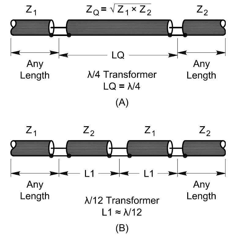
Examples of quarter-wave (A) and twelfth-wave (B) synchronous transformers. (Graphic courtesy of the ARRL)
The first reflection occurs when a wave from the transmitter (the incident wave) encounters the matching section. Since the impedances are different, part of the wave continues toward the load (which we assume is the antenna feed point) and the remaining wave is reflected back toward the transmitter. The ratio between the voltages of the incident and reflected waves is the reflection coefficient, ρ. If a wave encounters an open- or short-circuit, all of the wave is reflected and ρ = 1. If the impedance the wave encounters is the same as the impedance of the line it’s traveling through, such as in a matched load, there is no reflection and ρ = 0. For any other value of impedance encountered, ρ is between 0 and 1. ρ can also be used to calculate SWR = (1+ρ) / (1-ρ). (ρ is really a complex number, just like impedance, so what we really use to calculate SWR is the magnitude of r, correctly written as |ρ|.)
There is another change in impedance where ZQ meets Z2 and another set of reflections is generated. Some of the wave is reflected back toward the first junction and some is absorbed by the load. That might be the end of the story, but the new reflected wave encounters the junction of Z1 and ZQ, generating a new pair of waves: one continuing on toward the transmitter and one reflected back toward the load.
In the main feed line, we now have three waves adding together: the incident wave, the first reflected wave, and the wave that was reflected from the second junction at the load. The voltages of the waves all sum together, but the result depends on the relative phase of all three waves. That depends on the size of the impedance differences and the length of the matching section. This continuous series of reflections from both of the junctions continues forever until the transmitter stops transmitting. The reflections will get smaller and smaller until all of the wave’s energy is either absorbed by the load or dissipated as heat by feed line loss. This only takes a few cycles, which is a few microseconds at RF.
There is some ferocious math involved in calculating the end result of this infinite series of reflections. Skipping to the punch line, if the matching section happens to be λ/4 long and its impedance is the geometric mean of Z1 and Z2 as noted earlier, all the reflections in the main feed line cancel, the impedance at the input to the main feed line is Z1, and the SWR will be 1:1. Behold—the quarter-wave impedance transformer! (If you would like to see the full analysis of a Q-section, read “A Transient Analysis of an Impedance Transforming Device (The Quarter-Wave Transformer)” by Robert Lay, W9DMK, at www.qsl.net/w9dmk/qrtrwav4.pdf.)
Synchronous Transformers
The Q-section is an example of a synchronous transformer. Synchronous has multiple definitions, but the one that applies here is, “going on at the same rate and exactly together; recurring together,” from syn (together with) + chron (time) + ous (possessing or having the quality of). In this case, time is equivalent to the phase. Specifically, the phase of waves being combined in the transmission lines creates the impedance transforming effect. Not only that, but the same set of wave mechanics creates a match in the other direction, too, so the SWR looking toward the Q-section from the load is also 1:1! (This is the same principle behind anti-reflective optical coatings, although at much shorter wavelengths.)
It is important to note that an exact match occurs only at the frequency for which the Q-section is λ/4 long (or some odd integer multiple of λ/4) and if losses in the feed lines are low enough that they have an insignificant effect. Nevertheless, the Q-section provides an excellent match over several percent of bandwidth, good enough to use for a whole band at and above 7 MHz.
Q-Section Construction
The hardest part about making a Q section is often just coming up with the odd impedance transmission line! However, there’s no need to obsess over getting an exact match—any impedance within 10% of the exact value will give good results. 75Ω coax (RG-59) can be used to match impedances around 100 to 120Ω. Feed lines in parallel can be used to create a new feed line with half the characteristic impedance. For example, two pieces of RG-59 in parallel have an impedance of 75/2 = 37.5Ω, which can be used to match impedances around 25Ω to 50Ω cable.
Don’t forget that the electrical and physical lengths of transmission line are different. The length of a λ/4 piece of transmission line in feet is VF x 246 / f (in MHz), where VF is the velocity factor for the line. Cable with a solid polyethylene dielectric has a VF of 0.66. If your cable has a foam dielectric, the VF will be 0.78 to 0.83.
Tune the Q-section by shorting one end of the cable (twist the center conductor and shield braid together) and attaching the other end to your antenna analyzer, set to show impedance as R + jX. Ignore the SWR value and tune down in frequency from above the design frequency. Find the lowest frequency at which resistance, R, is a minimum. This is the frequency at which the line is λ/2 long, so divide by two to get the λ/4 frequency. Trim an inch or so at a time and repeat until the section is λ/4 long at the frequency you want.
You can check that the Q-section is working by terminating one end with a resistor having the same resistance as the load impedance. Verify that the SWR at the other end of the Q-section is close to 1:1. If you vary the frequency, you can find the Q section’s SWR bandwidth—the range of frequencies over which SWR is 2:1 or less. By substituting different values of terminating resistance, you’ll find out how much the termination can vary in either direction before SWR at the other end exceeds 2:1.
It’s not necessary to use coax connectors for the junctions of the transmission lines. If the installation is permanent, just solder the sections directly together. Make the shortest connections you can. Protect the junctions with multiple layers of high-quality electrical tape, such as Scotch 33+ or Scotch 88.
Twelfth-wave Transformers
The Q-section is really a special case of series-section matching. There’s no restriction (other than complexity) that there be just one matching section. In fact, the two-section variation shown in the figure is quite handy for matching two different impedances of transmission line, such as 50Ω coax and 75Ω hardline. Best of all, it doesn’t require any special transmission line impedances, only sections of line with the same impedances that are to be matched!
This configuration is referred to as a twelfth-wave transformer because when the ratio of the impedances to be matched is 1.5:1 (as is the case with 50- and 75Ω cables), the electrical length of the two matching sections between the lines to be matched is 0.0815 λ, quite close to λ/12 (0.0833 λ). You can use this trick to make good use of surplus low-loss 75Ω CATV hardline between 50Ω antennas and radios!