The dipole is the oldest antenna—Herr Professor Heinrich Hertz used a dipole in his 1888 experiments that confirmed Maxwell’s predictions of electromagnetic waves. The dipole (the word means “two voltage polarities”) is not unique to electrical phenomena. A guitar string vibrating at its fundamental frequency acts almost the same in radiating away acoustic energy. Replace motion of the string back and forth with the dipole’s magnitude of current flow and you can see the analogy.
Dipoles are also fundamental to radio! The very early dipoles were referred to as “Hertzian” antennas which were understood to be ½ wavelength long. At the very low frequencies and long wavelengths of early wireless, extending beyond 200 meters (1.5 MHz) into what we now refer to as Medium Frequency (300 kHz-3 MHz) and Low Frequency (30 kHz-300 kHz), putting up a full-size dipole was pretty much out of the question for hams. But then we were given the “worthless” wavelengths below 200 meters and suddenly, a full-size dipole was not so out of the question. (Read 200 Meter and Down by Clinton B. De Soto for the enchanting history of those days.) Along with the transition from spark to CW and the availability of vacuum tubes, the dipole was key (ahem) to making ham radio successful.
An Efficient Radiator
The primary reason the dipole became so popular was its effectiveness. The dipole is completely self-contained and is highly efficient with minimal losses. It doesn’t require enormous supporting structures, extensive ground screens, or special materials. An ordinary copper wire between two trees will work just fine, thanks, turning almost 100% of the applied RF energy from the feed line into radio waves. As long as the dipole is more than 1/10th wavelength high, ground losses in the soil underneath it are quite low as well.
While designed for use at its fundamental or half-wavelength frequency, the center-fed dipole will radiate effectively at any harmonic. The feed point impedance will vary quite a bit, changing from low values on the fundamental and odd harmonics to high impedance on the even harmonics. Ordinary coax works great for the low feed point impedances, which are usually between 30 and 100Ω (SWR ranging between 1.6 and 2:1.) However, coax becomes lossy for a high feed point impedance.
The usual solution is to use low-loss, open-wire feed line that remains fairly efficient at high SWR. Another popular solution is the end-fed half-wave (EFHW) that uses an impedance transformer at one end to match the antenna to coax. (The Par End-Fedz antennas at DXEngineering.com are typical.) The off-center-fed dipole (OFCD) is a compromise between the two, using a transformer to match the medium-value impedances found at one point along the antenna on several bands. (The MFJ-2010 is a good example of HF OFCDs.)
Elevation Pattern and Height
Regardless of how and where power is applied, the dipole is going to radiate basically the same signal. After all, feed point placement doesn’t change the length of the antenna. Like the guitar string again, we are just changing where we pluck it! In free-space, a half-wavelength (a.k.a. half-wave or ½λ or λ/2) dipole will radiate most of the applied energy broadside to the wire, forming the classic “doughnut” pattern. (A bagel is actually closer, with its smaller center hole, but let’s not quibble.)
I don’t know too many hams who operate from stations in free-space, at least on the HF bands, so we also have to consider the antenna’s height above ground. Why? Because some of the signal from the dipole causes current to flow in the ground, creating a reflection that is reduced by whatever loss from the resistance of the ground. That reflected signal combines with the signal directly from the dipole to create a pattern that often looks quite different from free-space pattern. (That perfect free-space dipole pattern shows zero radiation off the end, too, but a small amount is radiated, polarized oppositely to the antenna.)
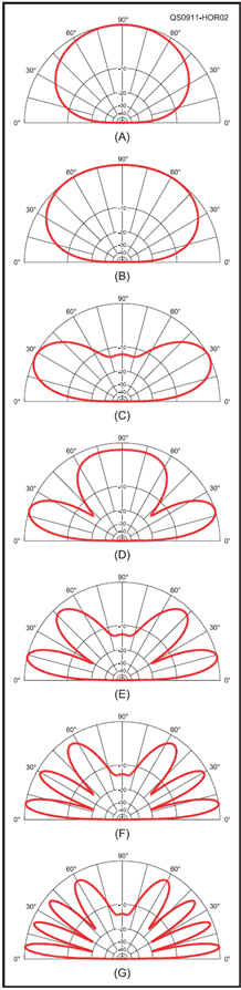
The figure above shows what happens to the cross-section of the dipole’s elevation pattern beginning at A with a height of 1/8thλ. The dipole is gradually raised to 1/4thλ (B), ½λ (C), ¾ λ (D), 1λ (E), 1-1/2λ (F), and finally 2λ (G). (The graphic is from the ARRL Antenna Book, 24th edition, courtesy of the ARRL.)
All About Angles
At very low heights (A and B), the dipole is radiating most of its signal in a cone aimed straight up and extending 30 degrees or more to each side. This is because at high elevation angles the ground-reflection signal reinforces the direct-radiation signal. As the antenna reaches ½λ (C), the two signals cancel in the vertical direction, but at 30 degrees of elevation they reinforce again, creating a much lower angle lobe. The bagel is getting squashed! As the height continues to increase, the cycle repeats with more and more side lobes created at different angles.
Taking advantage of these patterns is key to making the dipole a surprisingly effective antenna for “domestic” contacts. For North American stations, that means contacts around the U.S. and Canada primarily, depending on where your station is located. Most of these contacts at 7 MHz (40 meters) and higher frequencies will cover paths from 80o to 2,000 miles. For example, St. Louis to Denver is 850 miles, to Boston is 1,100 miles, and to San Francisco about 2,000 miles.
If you look at propagation tables for the various HF bands, you’ll find a surprisingly large fraction of the most likely arrival angles for these signals is 20 degrees or higher. Yet, if you look at the radiation pattern of typical 2- or 3-element Yagis at modest heights, the peak elevation angle is somewhat lower, between 10 and 20 degrees. For ground-mounted vertical antennas, it can be even lower. In other words, your low-angle antenna will miss out on high-angle signals!
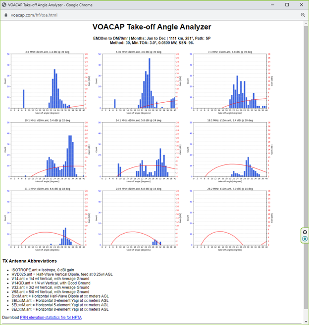
This set of graphs illustrate propagation between St. Louis and Denver from 3.5 MHz through 28 MHz (80-10 meters) in early September. In blue are the most likely arrival angles for signals on each band. In red is the elevation pattern for a ½λ dipole at 33 feet (10 meters) above the ground, abbreviated as “d10m.” (The assumption is that the dipole is oriented to give the best response on the specified path.)
If your low-angle antenna is optimized for working DX below 20 degrees (the middle of the horizontal axis) then most of the time, it’s going to miss a lot of the signals from Denver. It might hear Europe or Japan just fine, but Denver? Not so much. Since the dipole’s height is fixed, as frequency increases the dipole’s electrical height in wavelengths also increases.
You can see the dipole’s main lobe getting lower and lower as frequency goes up. From 40 through 15 meters, the dipole is going to receive signals from Denver a lot better than the low-angle antenna and the stations in Denver will hear your signal better, too. On 15 through 10 meters, it would be better for you to have an even lower dipole at 20 feet so you don’t miss the high-angle signals.
What’s the moral of the story? You need to pay attention to where the signals are coming from in elevation as well as in azimuth. Lower antenna pattern elevation angles are not always better and can be considerably worse! There are many instances when even the DX signals on HF are arriving at high angles. To capture these signals, a dipole or two at modest heights can be very handy.
Field Day, Sweepstakes, and your state’s QSO party are all great examples of where dipoles can make a big difference. Along with an omnidirectional vertical or beam, consider putting up a fan dipole or trap dipole at a compromise height of 25 to 30 feet. Make it easy to switch back and forth between your low-angle and high-angle antennas. You may be pleasantly surprised at what your “secret weapon” can do!
Generating Angle-of-Arrival Graphs
So how did I generate the above take-off-angle graphs? I used the free online VOACAP service which was developed for Voice Of America program and transmission planning. Start by selecting the start and end points of the path—move the red and blue pins or select locations from the TX QTH and RX QTH menus. Either accept the current date or enter a new date at the lower left. At the right, click the ANTENNAS button and select the antennas for each band. In the SETTINGS menu, you can enter any smoothed sunspot number (SSN) or a value of 1 will use the current SSN. Then click the green TO Angle button at the bottom of the window and wait while the host system completes the calculations.
You’ll find VOACAP to be a very handy planning and evaluation tool for any HF station needs. There are customized band opening and reliability charts for upcoming DXpeditions and a user’s guide available from the service’s home page. A quick-start guide is available here. Enjoy—but remember that no one has made a VOACAP-to-VOACAP QSO yet!