
(Editor’s Note: The following article is from the archives of experimenter, inventor, friend of the Ham Radio community, and founder of Clifton Laboratories, Jack Smith, K8ZOA (SK).)
This page presents measured data for selected audio transformers and shows how well the measurements permit the transformers to be modeled using LTSpice. The transformers selected are ones that might be considered for ground loop isolation when used with Softrock receivers, or when computer-based data transmission/reception programs are used with receivers or transceivers.
Transformer Modeling
I’m a firm believer in modeling circuits in computer simulation. It can save a great deal of time and error and enables many more “what ifs” to be conducted than can be done on the workbench.
At the same time, it’s important to not forget that a model is not reality. But, a good model, whether used with a computer simulator or as an aid to understanding circuit behavior is essential if one is to progress beyond the cut-and-try method of circuit design. I’m going to borrow a bit of this page from an article on RF transformers that I wrote for 73 Magazine some years ago.
Ideal Transformers
First, a quick review of ideal transformers. An ideal transformer has no losses; all of the power in the primary appears in the secondary. The relationship between the turns ratio N, primary voltage EPRI, secondary voltage ESEC, primary current IPRI and secondary current ISEC are governed by simple relationships:


In an AC circuit, impedance Z is the ratio of voltage to current. E, I and Z are, strictly speaking, complex, and may have both real and imaginary components. We’ll simplify things as much as possible and deal chiefly with the magnitude of E, I and Z.


The last equation is important; a transformer alters impedance by the square of the turns ratio.
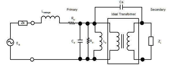
One simple, yet accurate, model of a practical transformer is shown in the figure below. Lp and Rp are the parallel inductance and resistance of the core, Rw is the winding resistance, Cd is the distributed capacitance and Lleakage is the leakage inductance. ZS and ZL are the source and load impedances. CS is the stray capacitance between windings. Note that all of these parasitic elements are shown in the primary circuit, although, of course, they are also found in the secondary. This is because the parasitic elements in the secondary can be moved to the primary by adjusting their values based on the ideal transformer turns ratio. This allows us to combine primary and secondary parasitic considerations into one set of components, simplifying computation considerably. .
For many purposes, we can simplify the model even further, considering the transformer to consist of an ideal transformer with a less than perfect coupling coefficient, and with series resistance in both the primary and secondary windings.
Simplified LTSpice transformer model. Note that the primary and secondary series resistance is added to L1 and L2 in a definition statement and does not show in the LTSpice schematic.
Let’s look at this transformer model in a bit more detail. It consists of two “coupled” inductors. The particular transformer this model comes from has two windings, a primary and a secondary with the same number of turns. The primary is wound with slightly larger diameter wire and has a bit lower resistance than the secondary.
L1 represents the transformer’s primary winding and L2 its secondary winding. L1 has a series DC resistance of 62.6 ohms and L2’s series DC resistance is 81.9 ohms. L1 has a measured inductance (with L2 being open circuited) of 0.6827 H, and L2 (with L1 open circuited) of 0.6806 H.
Comparing the simplified LTspice model with the first drawing, we see that the core loss, represented by Rp is ignored. Likewise, stray capacitance Cd and Cs are ignored. Rw is handled by the DC resistance, in this case appearing in both the primary and secondary windings, rather than being consolidated. Likewise, the primary and secondary inductance are separately stated and not consolidated into the primary side.
Instead of defining a separate “leakage inductance” in series with the primary, we take advantage of LTspice’s ability to handle mutual inductance and coupling coefficients, a subject worthy of further consideration.
Whether considered as a separate (but fictitious) “leakage inductance” or as a coupling coefficient less than 1.0, the effect is real. In any real transformer, less than 100% of the magnetic flux generated by the primary current cuts the secondary windings. Hence, some flux “escapes” or “leaks” out of the transformer.
Consider, for a moment, our first transformer model, with a short circuit on the secondary.
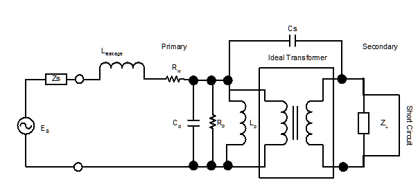
Since the ideal transformer in the model has no loss, the short circuit on the secondary is reflected back to the primary as a 0 ohm short circuit as well. Hence, Lp, Rp, Cd and Cs vanish from the model, and we are left with only the transformer’s leakage inductance Lleakage and its winding resistance, Rw.
Hence, if we measure the inductance of a transformer’s primary with the secondary short circuited (and vice versa) we can directly measure the leakage inductance.
In a perfect transformer, where 100% of the flux links the primary and secondary, Lleakage will be zero. In a well designed audio transformer, as we will see later on this page, Lleakage will be far less than 1% of primary inductance.
But, it’s equally valid to look at the transformer as two coupled inductors, the primary and secondary windings. As we recall from elementary circuit analysis, two inductors in series have a total inductance of Ltotal = L1+L2 only where the fields of the two inductors are uncoupled. If the fields are coupled, as in the illustration below, the total inductance of the two windings becomes more complicated.
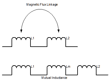
We define a new inductance, the “mutual inductance” that represents the contribution of L1’s field acting upon L2’s windings and vice versa.
If L1 and L2 are the inductances without mutual linkage, i.e., their self-inductances, then the total inductance L is: L = L1 + L2 ±2M M is the mutual inductance. It has a sign, in that if the fields of L1 and L2 add, the mutual inductance is in phase and L = L1 + L2 + 2M. If the fields oppose, then L = L1 + L2 – 2M. M is related to L1 and L2:

k is the “coefficient of coupling” and represents how well the flux from L1 cuts L2’s conductors and vice versa. If 100% of the flux of L1 cuts L2’s conductors and vice versa,
L1 and L2 are perfectly coupled and k=1.0.
If some of L1’s flux escapes L2 and vice versa, the two inductors are less well coupled and k is less than 1.0.
If we place the primary and secondary windings of our transformer in series, polarizing them such that their flux fields cancel, then we are measuring the inductance due to unlinked flux lines, which is exactly the same Lleakage we measue with the secondary shorted. Hence, it can be shown (I’m not going through the math here, however) that we are modeling the same physical phenomenon, leaking flux, whether we consider it as a separate series inductance Lleakage or as a coupling coefficient less than 1.00 in a program such as LTspice.
It may seem that we’ve placed undue emphasis on Lleakage, but to the contrary, Lleakage has a profound effect upon the transformer’s high frequency response, assuming the core is suitable for the frequency involved and the transformer is wound to minimize shunting capacitance.
Measuring Transformer Parameters
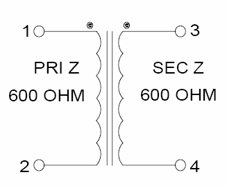
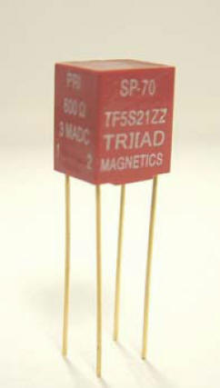
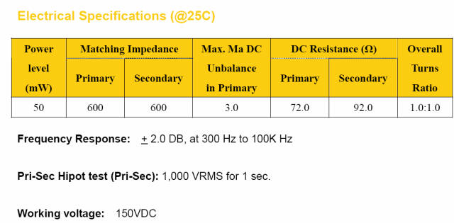
Let’s look at an actual transformer, a Triad SP-70 600 ohm : 600 ohm audio transformer. This is a high performance audio transformer, with a quoted response from 300 Hz to 100 KHz.
Winding Resistance
The simplest method of determining the winding resistance is a DC resistance measurement. Since the LTspice transformer model we use has separate primary and secondary windings, we will measure both.
DC Resistance (Ohms) Primary (1-2) Secondary (3-4) Measured 62.6 81.9 Specification 72.0 92.0
My measurements were made with an in-calibration Agilent 34410A digital multimeter, in 4-wire ohms mode, with Kelvin clips.
A more sophisticated measurement would be to measure the AC resistance, which reflects additional loss factors, including some core loss. We can derive the AC resistance from the inductance and Q, but it should be understood that the AC resistance is function of frequency and drive level, amongst other things, so AC resistance, if available, may only produce a small improvement to our transformer model.
Primary to Secondary Capacitance
Although we will not use it in our model, it is simple enough to measure the primary to secondary capacitance. Short the primary windings and the secondary windings and use a capacitance meter to measure the inter-winding capacitance.
Inter-Winding Capacitance
Primary to Secondary Measured 12.5 pF Specification Not quoted I used a General Radio 1658 Digibridge, with Kelvin extension clips to measure the interwinding capacitance. At the SP-70’s upper frequency limit of 100 KHz, 12.5 pF represents a bridging impedance exceeding 125K ohms. In most applications, this is a negligible effect.
Primary and Secondary Winding Impedance and Coupling Coefficient
Things became more interesting when I measured the SP-70’s primary and secondary inductance, mutual inductance and coupling coefficient. We make a series of six measurements for this calculation:
1. Lprimary with Lsecondary open circuit
2. Lprimary with Lsecondary short circuited
3. Lsecondary with Lprimary open circuit
4. Lsecondary with Lprimary short circuit
5. With Lprimary and Lsecondary in series aiding
6. With Lprimary and Lsecondary in series opposing
From this data, we calculate the coupling coefficient k two ways:
Method 1:
Step 1: Calculate M from measurements 5 and 6:

Step 2: From M, calculate k:

Method 2:
From measurements 1 and 2, calculate k

Where the Lp’ is the primary inductance with the secondary shorted (Lleakage in our very first model.)
As a check on the primary measurement, calculate k using the secondary measurements, 3 and 4.
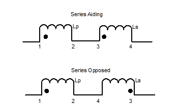
The correct polarity for measurements 5 and 6 is indicated by the phasing dots shown on the SP-70’s data sheet. If you don’t have a data sheet, connect the two windings in series and take data. Then reverse one winding and take the second measurement. It will be be obvious which is series aiding and which is series opposing.
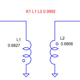
Here’s my data and calculated results, taken with a General Radio 1658 Digibridge, known to be accurate to within ±0.1%.
SP-70 w/ GR1658 Digibridge constant voltage
Input Measurements Lp 0.68270H
Ls open Ls 0.68060H Lp open
Laiding 2.17000H Lopposing 0.00098H
Lp 0.00118H Ls shorted Ls 0.00110H Lp shorted
By mutual inductance method:
M 0.5423H
k 0.7955
By open/short method
kp 0.9991
ks 0.9992
Geo Mean 0.9992
From experience, we know that a good audio transformer such as the SP-70 should have a coupling coefficient very close to 1.00. Hence, the open/short results are reasonable, if perhaps too good to be completely believable.
What happened to the mutual inductance method? A coupling coefficient of 0.8 is not to be believed. There’s no reason to believe the 1658 DigiBridge is in error, as it checks well against other equipment I have and against standard inductors.
The answer to this puzzle is that even in a good transformer, the core material has a nonlinear permeability and inductance varies with applied voltage. I’ve discussed changes in permeability with applied drive in conjunction with ferrite cores (click here to read) and the same thing is true with the material used in the SP-70 core.
It’s also necessary to know a bit about how the test equipment works. The 1658 DigiBridge applies a test voltage at 1 KHz to device under test and measures the resulting in-phase (I) and 90 degree out-of-phase (Q) current through the device. From this data the inductance and Q may be easily determined. The applied test voltage varies depending upon the inductance range. (The Digibridge also measures capacitance and resistance using the same technique.)
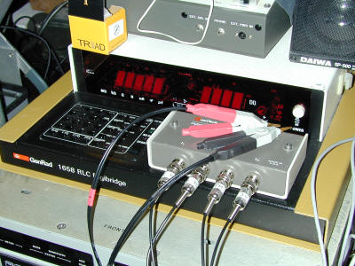
My 1658 Digibridge shown below with Quatech remote lead adapter and Kelvin clip test leads.
Using a battery powered Fluke 189 digital true RMS meter, I measured the following test voltage applied to the SP-70 by the 1658 DigiBridge operating in auto-range:
Test Condition 1000 Hz Voltage Across DUT Lprimary (20 mH-2 H range) 0.202 V Lsecondary (20 mH -2 H range) 0.202 V Lopposing (200 uH – 20 mH range) 0.209 V Laiding (2 H – 200 H range) 0.0323 V
Clearly the test voltage applied to the series aiding measurement is around 15% of the voltage applied to the other three measurements, a potential source of appreciable error if the inductance is a strong function of applied drive.
It is possible to engage “range hold” in the 1658, so I tried that first, holding the 2 – 200 H range, with the following results:
Input Measurements with Range Hold Lp 0.509H Ls open Ls 0.508H Lp open Laiding 2.121H Lopposing 0.00098H used old meas. M 0.530H k 1.04
This is clearly progress, but unfortunately k cannot exceed 1.00, so there’s still some error involved. Although range hold causes same test voltage to be applied, the error increases for out-of-range devices.
There’s a further error here as well�even if identical test voltages are applied for Lp, Ls and Laiding. The core permeability is a function of H, i.e., magnetic flux or ampere turns. With Lp and Ls in series aiding, the core is driven by twice as many turns, so that in order to obtain the same magnetic flux, we must reduce the current through the transformer by one half when measuring Laiding. Since inductance is proportional to N2, the series aiding configuration presents four times the reactance to the test voltage as does measuring either the primary or secondary alone. This means that we should measure the series aiding inductance with twice the test voltage used to measure the primary and secondary alone. (This calculation, of course, is for the SP-70 where the primary and secondary have the same number of turns. If the primary and secondary have different number of turns, a different test voltage ratio should be used.)
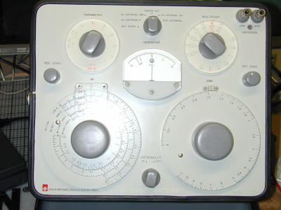
The 1658 DigiBridge doesn’t permit variable test voltage, so I set up the older manual GR1650B RLC bridge. It uses a 1 KHz test frequency, with an internal oscillator (external oscillators can also be used.)
The 1650B has an oscillator level control and, being a bridge type instrument maintains the same test voltage during bridge adjustment. Unfortunately, the 1650B has a ± 1% accuracy, making k measurements near 1.00 difficult at best.
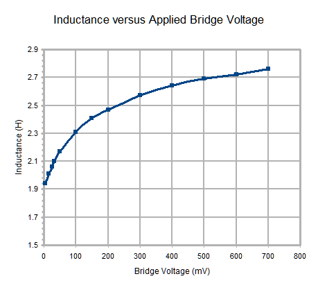
To get a sense of how much the inductance varies with drive, I connected the SP-70 in series aiding and measured the inductance versus drive level, adjusting the 1650B’s internal oscillator output over its usable range. As the plot below shows, inductance increases about 50% as the applied test voltage goes from 10 mV to 700 mV. When combined with the 1650B’s inherent 1% accuracy, an accurate k determination is still not easy.
The results are interesting.
SP-70 with GR1650B Constant I Drive
Test Voltage RMS Input Measurements Lp 0.67100H Ls open 250 mV Ls 0.67100H Lp open 250 mV Laiding 2.69000H 500 mV Lopposing 0.00104H 425 mV Lp 0.00104H Ls shorted250 mV Ls 0.00104H Lp shorted250 mV
By mutual inductance method M 0.6722H k 1.0018 By open/short method k1 0.9992 k2 0.9992 Geo Mean 0.9992
The test voltage has the necessary 2:1 ratio for Lp, Ls and series aiding. For series opposing, the test voltage is not as critical for two reasons. First, the series aiding error budget is 27 mH, at ±1% of the measured 2.69 H. Since the series opposing inductance is around 1 mH, any error in its measurement is insignificant compared with the series aiding error. Second, since the SP-70’s magnetic fields almost completely cancel in series opposing, the drive necessary to achieve comparable magnetic flux is unachievable and would, if applied, likely damage the transformer and the bridge.
Incidentally, if we use the -1% error bound for the series aiding inductance, we find the calculated k is 0.9922. It’s apparent that we are on the correct track, but the available instrumentation is not quite good enough to calculate k via the mutual inductance method. It is reasonably safe, however, to say that k > 0.99 based on the GR 1650B constant magnetic flux drive data.
One last point can be made. Calculating k from open/short measurements is discussed in Terman and Pettit’s Electronic Measurement, 2nd Ed., (1952) McGraw Hill, New York.
Terman notes that We should note that as k approaches 1, either method of measurement becomes increasingly difficult. I’ll leave it as an exercise for the interested reader, but consider what accuracy of inductance measurements are required to measure k = 0.99 with an accuracy in k of ±0.01, i.e., to have confidence that k is between 0.98 and 1.00. (The 1.00 part is easy, of course.)
Comparison of Model to Measured Results for SP-70
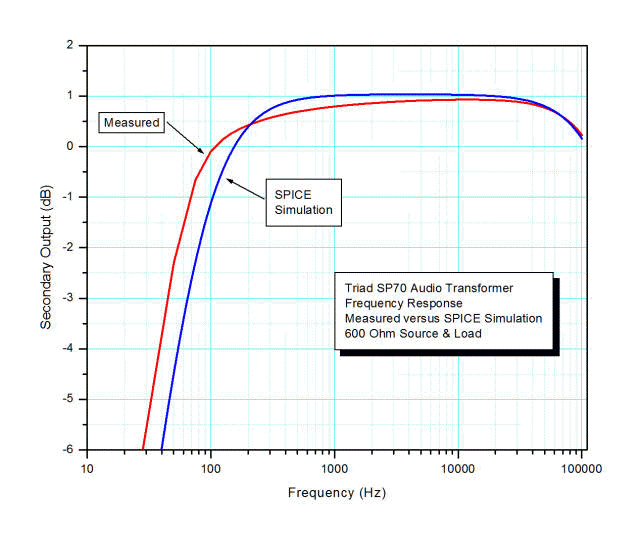
I ran frequency sweep data for the SP-70 using an automated setup, with a Telulex SG-100 function generator and an Agilent 34410A 6.5 digit digital multimeter, with both instruments under computer control. The final model of the test equipment and SP-70 transformer is as shown below. The 610 ohm driving impedance is a combination of the SG-100’s 50 ohm output and a 560 ohm 5% carbon film resistor. The 620 ohm terminating resistor is also a 5% carbon film type.
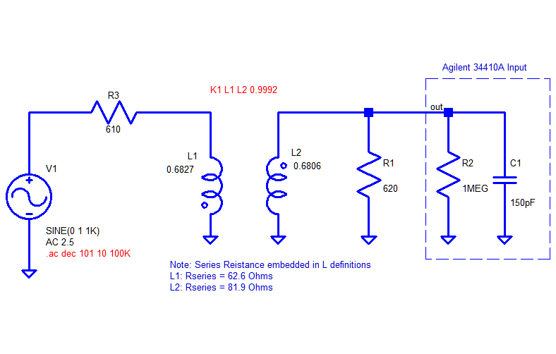
The measured and simulated data show excellent agreement over the range 100 Hz – 100 KHz, agreeing within 1 dB, and for the most part within 0.25 dB.
The worst divergence is below 100 Hz, where the SPICE simulation is pessimistic. Based on preliminary measurements, I believe this is a result of the SP-70’s core having increased inductance at lower test frequencies, i.e., the core’s permeability seems to increase with lower frequencies, below 100 Hz. At lower frequencies, inadequate magnetization inductance (Lm in the detailed model) rolls off the response.
To better simulate transformer operation in a Softrock receiver, or other similar designs where the transformer is driven by a low Z source and operates into a high Z impedance, I ran tests and models with a 50 ohm driving source and the transformer terminated in just the 34410A’s 1 Mohm shunted by 150 pF impedance.
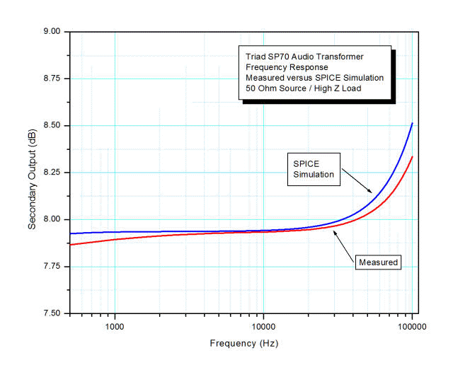
The agreement here is even more striking, being within 0.1 dB over the entire frequency range. When driven by a low impedance source, a transformer’s magnetization inductance becomes less important, and hence the low frequency response holds up better. (The data plotted cuts off at 500 Hz, but the agreement below this frequency is better than for the 600 ohm case.)
The rising response is due to resonance with the 34410A’s input capacitance and the SP70’s winding capacitance. In some circumstances, this rising frequency response can be used to offset roll off in other circuit elements.
Other Transformers
If you wish to model other audio transformers in LTspice, you may find the following data useful. All data was taken with a GR 1658 Digibridge, so the mutual inductance values suffer from the same drive-related errors discussed earlier.
Tamura TTC-264 datasheet at http://www.tamuracorp.com/clientuploads/pdfs/engineeringdocs/TTC-264.pdf Tamura TTC-264
Input Measurements L1 0.17693H L2 open L2 0.17467H L1 open Laiding 0.6734H Lopposing 0.005014H L1 0.006241H L2 shorted L2 0.006776H L1 shorted
By mutual inductance method M 0.1671H k 0.9505
By open/short method k1 0.9822 k2 0.9804 Geo Mean 0.9813 Triad TY-145
Input Measurements L1 0.5117H L2 open L2 0.5121H L1 open Laiding 1.8438H Lopposing 0.003841H L1 0.003933H L2 shorted L2 0.003899H L1 shorted
By mutual inductance method M 0.4600H k 0.8986
By open/short method k1 0.9961 k2 0.9962 Geo Mean 0.9962
In both cases, I would use the open/short data for modeling for the reasons developed above. It likely slightly overstates the coupling, but the mutual inductance data is clearly in error for the reasons given earlier.