(Editor’s Note: The following article is from the archives of experimenter, inventor, friend of the Ham Radio community, and founder of Clifton Laboratories, Jack Smith, K8ZOA (SK).)
One project I’ve been occupied with, likely to be available as a kit or assembled unit, in the next few months, is an AM broadcast band rejection filter. My friend Ron, K8AQC, lives in a suburban Detroit location with extremely strong AM broadcast signals and this summer I built a one-off filter to pass frequencies below 400 KHz and above 1.8 MHz but to significantly attenuate signals in the 500-1700 KHz AM medium wave broadcast band.
The filter I built for Ron worked so well that I thought it might have use for others suffering from high level AM broadcast band signals. I’ve laid out a printed circuit board and have now assembled three filters and thought the design decision around inductor design might be of interest.
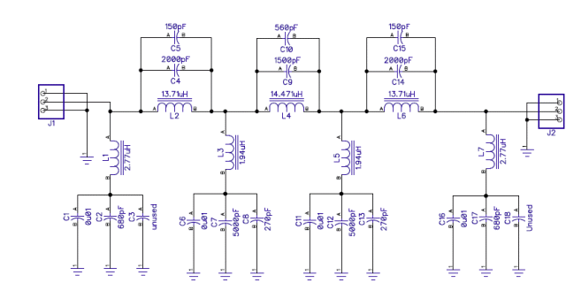
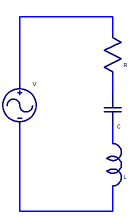
The figure below shows a near final schematic of the filter. I’ve made some small component value changes, but for the purpose of this discussion, the changes are not significant.
My target is for the band reject filter to have less than 1 dB attenuation outside the stop band, subject to the fact that it’s a Chebyshev design so it will have the usual ripples in the passband that are the price paid for the Chebyshev’s superior roll off compared with a filter without passband ripples, such as a Butterworth. I’ve set the design parameters for 1 dB ripple, so with the added loss due to finite Q components, we can expect to see a few ripples of 1.5 dB or so loss within the passband.
.My goal is to have the passband meet this performance target over a rather wide frequency range, 10 KHz to 100 MHz. (As shown later on this page, the goal is met.) This brings up a major design choice: what inductors to use. Looking at the filter schematic, we see three parallel resonant sections with inductors around 14 µH and four series resonant sections with around 2.5 µH inductors.
Superficially, therefore, we need our inductors to meet several requirements:
- Constant inductance, more or less, from 10 KHz to 100 MHz
- High Q over this range
- No self-resonance effects
- Small physical size to keep cost down
In fact, of course, there are no physically realizable inductors that meet all four of these requirements. Before departing on a quest for physically impossible parts, we first should carefully look at the purpose of the filter and how that purpose interacts with physically available parts.
For several good reasons, our search will focus around toroidal inductors:
- Provides reasonably high Q in small physical size
- To a large degree (but not perfectly) self-shielding with much reduced unwanted magnetic coupling amongst the inductors
- Reasonable price
- Able to be constructed by kit builders, potentially at least, depending on the degree of precision required and the builder’s available test equipment.
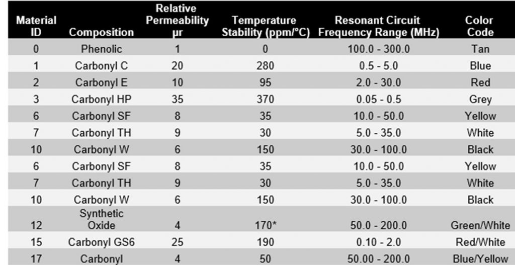
Of the toroid core materials readily available, we have two families:
- Powdered iron
- Ferrite material
Powdered iron parts are commonly identified by hams by a Tnn-x identification where nn represents the core’s outer diameter in units of 1/100th of an inch and x identifies the particular “mix” or composition of the iron and binder in the core.
Ferrites are chemically complex formulations with iron, zinc, nickel and manganese, amongst other things. In amateur parlance, these are identified as FTnn-xx where nn is again the core outer diameter in units of 1/100th of an inch and xx identifies the mix.
The Tnn-x and FTnn-x identifiers were developed by a particular distributor and do not represent the actual core manufacturer’s part numbers, but these shorthand identifiers have become embedded in the literature and, in fact, are rather handy, so we’ll use them here.
From the leading manufacturer of powdered iron cores, Micrometals, the key parameters of its various mixes are:
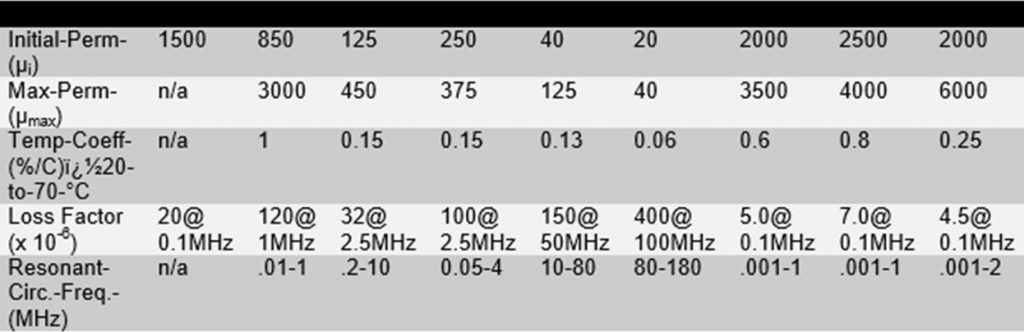
Similar information for the common ferrite cores from the leading ferrite manufacturer, Fair-Rite, is provided below.
This is a lot of information – what do we make of it?
It should be apparent that our belief that no single material is suitable for the frequency range 10 KHz – 100 MHz is apparent in the data. But, do we really need a material that works uniformly over this frequency range? Let’s look at our filter circuit. (I’ll provide high level arguments with limited math here – detailed mathematical circuit analysis will be left to the interested reader.)
One other point is that the discussion below suggests that the filter can be considered as independent series and parallel resonant circuits. That’s a gross oversimplification if not an outright error, but has enough validity to make the exercise useful in understanding the choice of core materials.
At frequencies below a few MHz all the filter tuned circuits are operational. In the AM broadcast band, 530 – 1700 KHz the three parallel tuned circuits (L2, L4 and L6 with associated capacitors) should provide a high impedance path, whilst the four series tuned circuits (L1, L3, L5 and L7 and associated capacitors) form a low impedance path shunting this frequency range. The impedance (both parallel and series) is a function of resonant circuit Q (dominated by the inductors, since we can use polystyrene capacitors with very high Q) so we need all inductors to have high Q performance in this frequency range. The reject band depth is a function of the component Q.
Consider next what happens at relatively high frequencies, say 10 or 15 MHz up through 100 MHz or more. The parallel tuned circuits centered a round L2, L4 and L6 are way outside their resonant frequency range, and their impedance is dominated by the shunting capacitance. At 15 MHz, for example, the 2000 pF or so capacitors in this section of the filter have an impedance around 5 ohms. If L2, L4 and L6 are not particularly good inductors at these frequencies, there is only a small change in the impedance of these LC circuits. Hence, we can accept even a major drop in inductor performance of L2, L4 and L6 if required.
The four series tuned circuits associated with L1, L3, L5 and L7, however, must still retain a reasonably high impedance throughout the entire passband range. Otherwise, the desired signal frequencies will be shunted to ground and hence increased attenuation results. However, if these series resonant circuits collectively have an impedance of a few hundred ohms, the resulting passband loss may be acceptable. So we can accept some poorer performance of L1, L3, L5 and L7. (Remember as I mentioned at the outset, this is a grossly oversimplified analysis of how the filter actually works.)
In sum, therefore:
- At frequencies up to a few MHz, all seven inductors must provide good performance, high Q and reasonably constant inductance with frequency.
- At higher frequencies, say above 10 MHz, we can accept some fall off of performance in L1, L3, L5 and L7.
- At higher frequencies, say above 10 MHz, L2, L4 and L6 can have rather significant performance impairments without harming our filter’s overall performance.
- There’s still a limit how bad all these inductors can be without excessive insertion loss, of course.
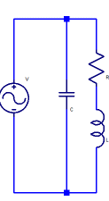
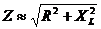
To help quantify these comments, we can look quickly at the math involved. The impedance Z of a series RLC circuit such as the one shown above is:
where XL is the reactance of inductance L at frequency f: XL = 2πfL
and XC is the reactance of capacitor C at frequency f XC = 1/2πfC
R is the series resistance representing losses in the capacitor and inductor. If the capacitor’s loss is small compared with the inductor’s losses (as is quite often the case) the relationship between R and the inductor Q is:
R = XL/Q or R = 2πfL/Q
At the resonant frequency XC = XL, so Z reduces to simply R. For a 2.5µH inductor, with a Q of 200 at 925 KHz, for example, R is 2*π *0.925×106 * 2.5 x 10-6 / 200 = 0.07 ohms.
In our filter design, the L1, L3, L5 and L7 circuits are resonant around 925 KHz, at which frequency XC = XL. At 10 times this frequency, or 9.25 MHz, XL is 10 times as large as its value at 925 KHz and XC is 1/10th its value. Returning to our equation for Z in terms of R, XL and XC, we note that (XL – XC) ≈ XL, with sufficient engineering accuracy. The impedance Z is therefore:
Recasting this equation in terms of Q, we find:
which may be further simplified to:
This is an interesting result from which we may draw several conclusions, reinforcing mathematically my earlier observations:
- With a Q as low as 3, Z is within 5% of the value it has for infinite Q
- As Q diminishes, Z increases. Since the high frequency passband employs the series tuned circuit in shunt, increased Z is actually beneficial, not harmful, to the filter’s loss.
Hence, at frequencies significantly above resonance, not all that important in determining the impedance of the series circuit. We could also extend this observation to note that even if the inductance drops with frequency due to changes in the core material’s permeability with frequency, for example, Z may not change all that much. Of course, a radical change in inductance with frequency, such that the RLC circuit becomes resonant at some elevated frequency would be a problem.
A numerical example may help. Take the 2.5 µH inductor used in the earlier computation, but assume the Q drops to 20 at 9.25 MHz. What is Z?
- With Q=infinity, Z= 145.298 ohms
- With Q = 20, Z = 145.480 ohms
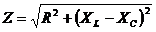
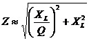
We can do the same analysis for the parallel resonant RLC network shown above, where the magnitude of the impedance is.
ω is the frequency in radians per second, ω=2πf where f is the frequency in Hz.
Amazing that moving one component makes such a difference in impedance complexity, isn’t it? However, the equation is not as difficult to analyze as it might appear.
What is the impedance of this circuit at “resonance”? Before we can answer that question, we first have to decide what is “resonance.”
There are three possible definitions of resonant frequency the parallel circuit:
– The frequency for which the circuit impedance is maximum; – The frequency for which the impedance is purely resistive (unity power factor); and – The frequency corresponding to series resonance, i.e.,

If R is not too large compared with XL, which is another way of saying that L has a reasonable Q, the three possible resonant frequencies become sufficiently close that we may treat them as identical and use the simplified series resonant formula.
In the high Q case, therefore, after a bit of algebra, at resonance:
RS is the series resistance of the inductor.
From this, we observe at resonance:
- Impedance is directly proportional to the inductor Q (remember we assume no loss in the capacitor.)
- The smaller C is, the higher Z is.
So much for resonance
At resonance, we wish the impedance to be large, as it reduces the stop band signal level, the purpose of our filter, after all. But what about frequencies far above resonance? If we assume R is small compared with XL, the impedance of the parallel resonant circuit is approximately:

L/C is a constant (assuming L is not varying with frequency) so as the frequency increases, Z diminishes. This is because ωL = ωC at resonance and hence as ω increases (ωL -1/ωC) also increases reducing Z. (The same is true for ω decreasing far below resonance; (ωL -1/ωC) also increases because the 1/ωC term dominates.)
After all this work, which has taken me far longer to write than to consider during the design process, we conclude that:
- L2, L4 and L6 can be ferrite material, if the selected ferrite holds reasonably constant inductance up to 10 MHz or so (about 10 x the resonant frequency) and if the material’s Q is reasonable over this range.
- L1, L3, L5 and L7 can be powdered iron, since they should retain reasonable Q well above 10 MHz.
Which ferrite and which powdered iron to use is the next question.
Looking at the table, the only reasonable choice is Type 61 material. The manufacturer suggests it is suitable for resonant circuits over the range 200 KHz to 10 MHz.
We have a wider choice for the powdered iron cores. I’ve decided to use Mix 7 (white) material, but Mix 2 (red) would likely do nearly as well.
To obtain a sense of how these two core solutions work, I wound test inductors of approximately 14 µH:
- 15 turns, no. 24 AWG magnet wire on an FT50-61 core, nominal inductance at 2.5 MHz of 13.8µH, Q = 200 as measured on an HP 4342A Q-meter.
- 58 turns, no. 30 AWG magnet wire on a T50-7 core, nominal inductance at 2.5 MHz of 14.6 µH, Q = 184.
- 51 turns, no. 28 AWG magnet wire on a T68-7 core, nominal inductance at 2.5 MHz of 14.3 µH, Q = 220.
The figure below shows the variation in inductance of these three test coils over the range 800 KHz to 9 MHz, measured with an HP 4342A Q-meter. The 4342A is an analog instrument with a quoted accuracy of ±3% for inductance and ±7% for Q. At 15 µH, ±3% corresponds to ±0.45 µH, so it’s reasonable to ascribe a great deal of the variation in the measured inductance up through 7 MHz or so as instrument error. (If the inductance is actually constant over this range, the observed instrument error is around ±0.9%.)
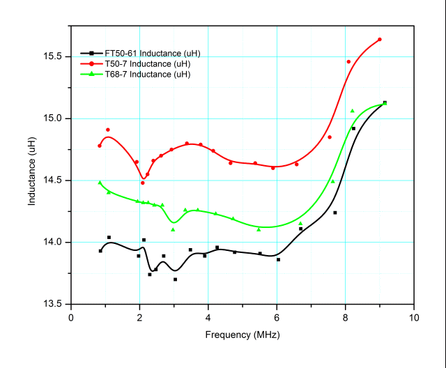
The data shows that either the ferrite mix 61 core or the -7 powdered iron mix provide quite reasonable inductance stability over the measured range. At frequencies above 7 MHz or so, the observed inductance rises for all three test inductors. This is almost certainly due to distributed capacitance between winding turns. In fact, if we assume that the inductance below 7 MHz is the “true” inductance, it’s possible to estimate the distributed capacitance of the windings:
- T68-7: 1.25 pF
- T50-7: 1.38 pF
- FT50-61: 1.91 pF
The plot below shows the indicated Q for the three test inductors over the same frequency range. (No correction for distributed capacitance is made in the data.)
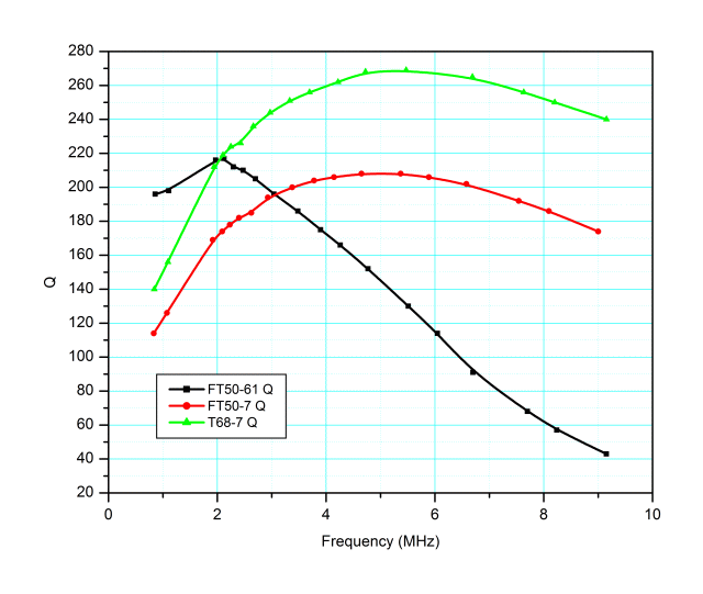
Based on data from the manufacturer of the powdered iron material, Micrometals, the two powdered iron specimens more than meet their specifications.
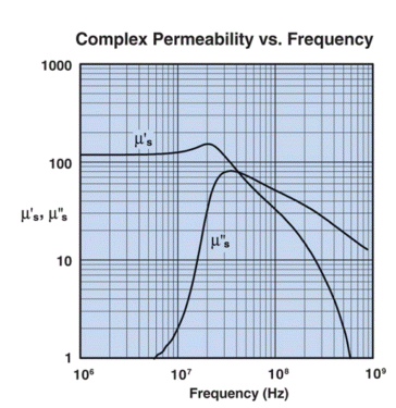
The type 61 ferrite material shows a considerable drop in Q with increased frequency, which again can be seen if the manufacturer’s specifications are examined. The plot below is from Fair-Rite’s catalog and shows how mix 61’s “complex permeability” varies with frequency. For our purposes, I’ll just say that the core material’s intrinsic Q is the ratio of u’/u”. At 10 MHz, for example, Fair-Rite data shows u’ is 125 whilst u” is 2, providing an intrinsic material Q of 62. The “intrinsic Q” is, of course, degraded by copper loss in the winding and other considerations and therefore represents the maximum Q that one might observe.
The main benefit from using a ferrite core for L2, L4 and L6 can be found when the number of turns is examined; it’s much easier to wind 15 turns of rather large wire onto a core than 58 turns of very small wire.
To see how much effect the core material had on actual filter performance, I built three band reject filters, identical except for how L2, L4 and L6 were constructed. L1, L3, L5 and L7 in all three filters are wound on T50-7 cores.
- Filter 1: L2, L4 and L6 are wound on T50-7 cores
- Filter 2: L2, L4 and L6 are wound on T68-7 cores
- Filter 3: L2, L4 and L6 are wound on FT50-61 cores
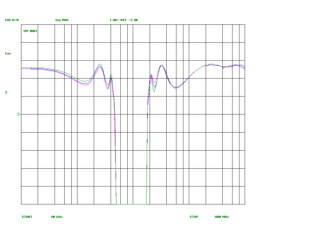
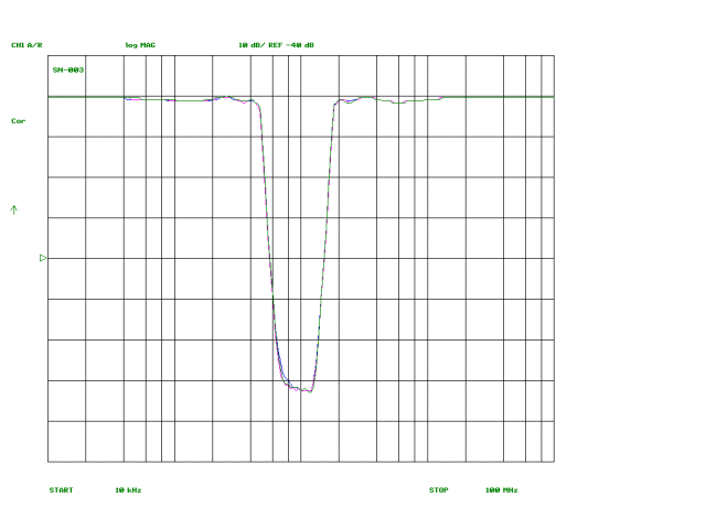
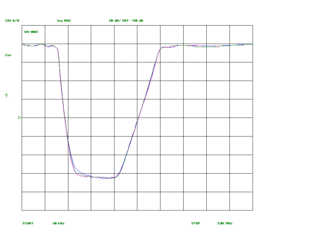
The plots below show the measured response curves for the three filters, plotted onto single graphs. The difference between the three is negligible, amounting to fractions of a dB in the passband and, at most, a dB or two for a small portion of the reject band. Accordingly, the choice between FT50-61 and T50-7 or T68-7 cores for L2, L4 and L6 can be made on the basis of cost and convenience without concern over performance concerns.
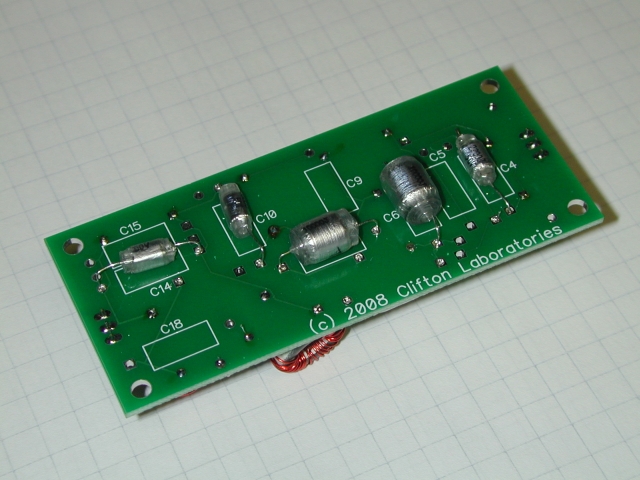
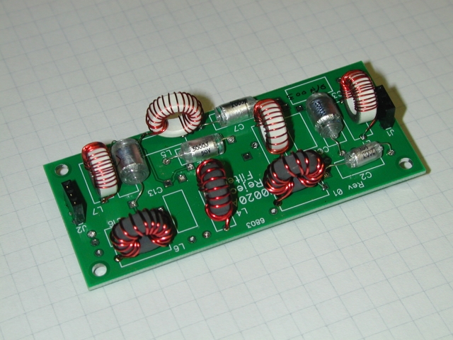
The photos below show the filter built with FT50-61 (L2/L4/L6) and T50-7 (L1/L3/L5/L7) parts.